L'état du blog: 2022

Another calendar year down; also another annus horribilis. Let’s review what happened in this Crummy Little Blog That Nobody Reads (CLBTNR), and studiously avoid the more daunting task of reviewing 2022.

No Posts for 3 Weeks?!

Yes, it’s been that long. A combination of depression and post-COVID-19 brain fog (still lingering from last summer) has made everything hard. And I mean everything.

Trust me, I’ve got browser windows full of tabs of references on things about which I want to write. Or more correctly, want to have written, the actual writing being a bit beyond my capabilities at the moment.

And the comments are still disabled. I could follow the detailed Staticman tutorial to get it hosted on Heroku. But when Heroku folded their free accounts, there were only vague assertions about how it was doable on other hosting services. Yes, if you’re a full-time cloud-computing person, that’s enough. But if you’re not, there’s a lot of figuring out to do… and my figure-outer is on the fritz.

In the meantime, there is, and always has been, an email link at the top of every page (the little envelope hieroglyph).

Still, there’s some medication that might kick in any day now. And the brain fog lifts after a median time of 6-9 months, which means February to May.

It would be nice not to have to rely on brute-force stubbornness so much, wouldn’t it?

When the geeks count time by the kalends

(Yes, I’m going to repeat that sub-titular joke every year until somebody gets it. Probably even after that.)

Fiat blog was on 2020-Jul-01, my first day of retirement. Just now, my second full year of retirement blogging ended on 2022-Dec-31.

According to the TimeAndDate.com duration calculator, 914 days have elapsed total, 365 of which were in calendar 2022 proper. (Or 78,969,600 seconds. I remember in my early 30s when I realized I was a bit over 1 gigasecond old. That mattered more to me than turning 30. Aging to 2 gigaseconds in my sixties was less of a big deal. Making it to 3 gigaseconds is not impossible, but low probability.) So we’ve been writing this Crummy Little Blog That Nobody Reads for almost exactly 2 1/2 years:

The year-end is a time for retrospection and introspection. And since it’s the bi-sesqui-blogiversary, let’s see how things have gone. For that purpose, I’ve written a little R script to analyze post/comment/hit statistics and test for trends over time, the relationship between comments and hit counts, etc. ^[1] (Excluding this post itself, of course, for obvious reasons!) It’s been revised extensively since last year, e.g., with distribution modeling for the hits per post, q.v.

The results of this script (transcript and spreadsheet) are available in the Notes & References below for all 30 months as an omnibus dataset. ^[2] In my (mildly) cognitively diminished state, I’m not up to doing the year-by-year breakdowns.

Conclusion: Calculemus!

Frequencies of posts, comments, and hits

So first let’s use the script’s output (saved in spreadsheets in the Notes & References) to get an idea of how many posts and comments there were in 2020 and 2021, and some idea of the average rate. From the transcript, we can extract the nifty little table shown here.

• Recall that we started blogging in mid-2020, so only half the days of 2020 are available. So the Null Hypothesis of constant rates is: twice as much activity in 2021 and 2022 compared to 2020.
• We’ve posted consistently more frequently than the first year, even with my recent 3 week stand-down.
• The comments per post remain about constant, i.e., low. On the other hand, comments have been disabled for 2 months now, until I get the mental oomph to go fix it; so maybe the comment rate would be a tad higher if we were to allow for that?

Conclusion: This is still a blog you can keep up with by reading once a week. Also, for some mysterious reason I get more comments via email than the comment system (when it’s working, of course!).

Hits and comments in relation to time

That’s been mostly about writing posts. What about reading?

To investigate readership, we’ll next look at the post hits vs time (regrettably including my own looking at the posts searching for errors and things to rephrase), and comments vs time.

Modeling the Distribution of Post Hits

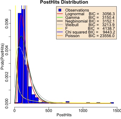
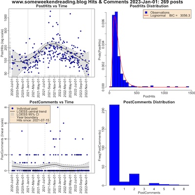
This year, though, we’ve done a bit of distributional modeling of the hits per post. Shown here is the histogram of hits, showing the dominance of low-hit posts along with a long tail of outliers that somehow got more exposure. We’ve overplotted that with best-fit distributions (using the fitdistrplus package in R).

We’ve characterized each candidate distribution by the Bayes Information Criterion (BIC) for how well it fits the data. This is a parameter-penalized negtative log likelihood, i.e., it accounts for how many parameters you spend on complexity and rewards you for having better log likelihood. Smaller is better.

Now… you’re not supposed to do this!

Shopping for distributions, even with an appropriately penalized likelihood like BIC, is a no-no. I should build a probabilistic model of how hits arrive, and fit that rather than just trying easy things. But that’s hard: recent posts are exposed to the web for less time, early posts were mosty unread except for people now looking through my back-catalog, and so on. So I’m going to grit my teeth here and be empirical at the expense of principle, something that kind of grates on my brain.

I decided to salve my conscience by testing all distributions that had reasonable properties were feasibly available to me:

1. Univariate,
2. Unimodal,
3. Bounded below at 0 (after suitable transformation),
4. Capable of sufficient skewness to fit a long right tail, and
5. Reasonably easily available in R and the fitdistrplus package.

The obvious candidates were lognormal, Gamma, negbinomial, Weibull, and Poisson. A few others were easily available, but I ruled them out based on the criteria above:

• uniform as not unimodal,
• Cauchy, normal, and $t$ as not bounded below at 0 and not having right-skewness for any parametrization,
• geometric as a special case of negbinomial,
• exponential based on observed shape different from the empirical histogram (mode always fixed at 0, not a finite value as observed in the data),
• Beta because its values have to be in [0, 1] and it felt artificial to transform that too drastically, and
• binomial due to convergence problems and for large values it’s Poisson anyway.

After a bit of a wrestle, I was able to guess optimizer starting values for the $F$ and $\chi^2$ distributions as well, though the resulting fit parameters look pretty absurd. Going down the list in order of increasing BIC (i.e., from best to worst):

• Lognormal (red curve): Actually pretty good! By all 1 objective statistica and 3 qualitative observables: objective BIC, and noting it fits the peak correctly, the width correctly, and respects the long right tail. I have no especial theoretical reason to favor lognormal, but empirically I like the result.
• Gamma (green curve): The peak is too low and the width is too wide. Otherwise, not terrible.
• Negbinomial (black curve): Essentially identical to Gamma. I realized after the fact that there’s a change of variables that makes Gamma and negbinomial the same, and the optimizer found this.
• Weibull (gray curve): I had high hopes for this, since it’s used in Extreme Value Theory, and here we have empirical data with a long right tail! Alas, not only is the BIC in 4th place, but the fit is not so good either: peak too far to the left and way too low, as well as both left and right tails too heavy.
• $F$ (yellow curve), $\chi^2$ (blue curve), and Poisson (orange curve): All hopeless, both by BIC and visual fit to the data.

Conclusion: Empirically, at least, post hits are more or less lognormaly distributed.

What the Post Hit/Comment Data Says

Here’s the hits vs time and comments vs time for the last 2.5 years (click to embiggen). The 4 plots are:

1. Top left: Hits vs time. The horizontal axis is time; the vertical axis is the number of hits on a log scale. Each blue point is a post. The black curve is the LOESS curve (sort of like a local curve fit); the gray band is the 95% confidence interval on the LOESS curve. The vertical dashed line is when hit tracking was turned on; hits before this date represent people looking through the back catalog of posts.
2. Top right: Histogram of hit counts. This gives you an idea of the probability distribution of hits. The distribution shown in red is the best-fit lognormal distribution.
3. Lower left: Comments vs time. The horizontal axis is time; the vertical axis is number of comments (linear scale). Each blue point is a post. The LOESS curves are as previously explained.
4. Lower right: Histogram of comment counts. This gives you an idea of the probability distribution of comments per post. There are so few comments we didn’t fit a distribution here.

The interpretation seems pretty clear:

• The surge in hits in 2021 Q3 was temporary. This is when I was live-blogging FDA hearings, and attracted some interest from nervous nerds like myself. They moved on when that was over. (I joked last year with a friend who coaches startup founders about getting on their “S-curves” that I was probably building the world’s most useless S-curve. Yep… pretty useless.)
• Most posts get $O(10^2)$ hits (including people looking at the back catalog of old posts), and comments are rare.

The lognormal distribution becomes normal when you take the log, so the 2 parameters are $\mu$ and $\sigma$ of the log number of hits. Here we got a mean and standard deviation of log hits, with uncertainties, of $\mu = 4.86 \pm 0.03$ and $\sigma = 0.53 \pm 0.02$.

Conclusion: Still a crummy little blog that nobody reads, unless I write about an FDA hearing for medications against life-threatening pandemic diseases, and advertise that fact in the comments section of a high-traffic blog.

On the Relationship Between Post Hits & Comments

Again we entertain the hypothesis that posts with more hits might get more comments, though this year that (putative) relationship is likely disrupted by the comments being broken for more than a month. Still, let’s examine the unsupervised bicluster and the supervised semi-log regression we did last year.

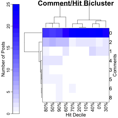To investigate such a relationship in 2021, we’ll first do an exploratory bicluster of comment counts vs hit counts (top figure), and then a linear-log regression of comments on log hits.

• The bicluster is shown on top:
  • The color shows the number of posts with a given number of hits and number of comments.
  • The rows are just the number of comments.
  • The hits have been reduced to a rank, i.e., a decile. This is to take care of outliers, i.e., the one post that got $O(1200)$ hits. (This plays the same role as the log transform in the regression, q.v. They are shown in the columns.)
  • The row and column dendrograms permute the rows and permute the columns until the ones that most resemble each other are adjacent. The length of a leg of the dendrogram indicates the statistical significance of the split.
  • Comment dendrogram (rows): Here the story is brutally clear: the 0-comment row stands out with most of the posts, and any number of hits above 0 makes them all look almost identical.
  • Hit decile dendrogam (columns): Basically there are only 2 groups here. On the left branch are the posts that have a long tail of comments beyond 0-2, and on the right those that do not.
  • We conclude that the 0-comment posts stand apart, and there is weak to no evidence of more hits leading to more comments, as the 2 column clusters show opposite results!
    
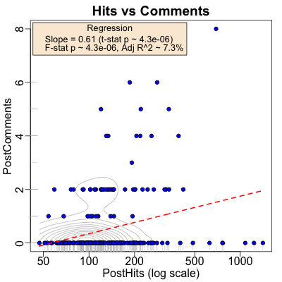
• The linear-log regression is shown on the bottom:
  • Each post is a blue dot.
  • The horizontal axis is the number of hits, on a log scale. The rug on the horizontal axis gives you some idea of the (log) density of hits.
  • The vertical axis is the number of comments for each post. The rug on the vertical axis is uninformative, as there are only 7 levels.
  • The gray curves gives you an idea of the joint density (from kernel density estimation by convolution with a gaussian of appropriate bandwidth). It definitely says most of the probability is concentrated along the horizontal axis, i.e., 0 comments.
  • The red line is the regression line.
    • On the one hand, it is statistically significant, i.e., probably real: the $F$-statistic for the overall regression has $p \sim 4.28 \times 10^{-6}$, and the $t$-statistic for the slope coefficient does as well.
    • However, the strength of the prediction is miserable with an adjusted $R^2 \sim 7.3\%$, i.e., log hits explains only 7.3% of the variance in comments.

Call:  
lm(formula = PostComments ~ log(PostHits), data = postData)  
 
Residuals:  
    Min      1Q  Median      3Q     Max  
-1.9598 -0.5689 -0.3343 -0.0841  6.4744  
 
Coefficients:  
              Estimate Std. Error t value Pr(>|t|)  
(Intercept)    -2.4601     0.6341  -3.880 0.000132 ***  
log(PostHits)   0.6095     0.1298   4.694 4.28e-06 ***  
---  
Signif. codes:  0 ‘***’ 0.001 ‘**’ 0.01 ‘*’ 0.05 ‘.’ 0.1 ‘ ’ 1  
 
Residual standard error: 1.152 on 267 degrees of freedom  
Multiple R-squared:  0.07624,	Adjusted R-squared:  0.07278  
F-statistic: 22.04 on 1 and 267 DF,  p-value: 4.28e-06  

It seems clear that a naïve linear model is still useless here. While the nonzero comment points may have a mild trend, the 0 point comments drag the regresion into sillyspace. Perhaps something like tobit regression would be more appropriate?

But if we back up a bit and try to be a little less model-based, we find that there is a statistically significant relationship between hits and comments, both numerical Pearson correlation and rank Speaerman correlation:

	Pearson's product-moment correlation

data:  postData$PostHits and postData$PostComments
t = 2.8179, df = 267, p-value = 0.005195
alternative hypothesis: true correlation is not equal to 0
95 percent confidence interval:
 0.05139208 0.28377561
sample estimates:
      cor 
0.1699455 

	Spearman's rank correlation rho

data:  postData$PostHits and postData$PostComments
S = 2470816, p-value = 7.864e-05
alternative hypothesis: true rho is not equal to 0
sample estimates:
      rho 
0.2383758 

Both have nice $p$-values, but small(ish) correlations. So that’s consistent with a real, but weak relationship.

Conclusion: Most posts get 0 comments. While there is statistical significance to a putative comment/hit relationship, the strength of prediction is essentially nothing. A more signficant model involving cutoffs, like tobit regression, will be fun to explore at in year-end post for… some future year.

The boring nature of spam and the (blessedly infrequent) nastygrams

There’s still lots of spam, mostly in Russian. I haven’t broken it down by year (perhaps I will do so next year?), but overall nearly every comment submitted is spam. Of course, having the comment system break was a particularly strong response to spam!

So the detailed comment source analysis of previous years is probably not apt here.

Google search console and its discontents

We can also use Google Search Console to see things like how often we come up in Google searches, what the search queries were, how often people clicked through, and what other web pages link to us.

Search appearances and click-through rate

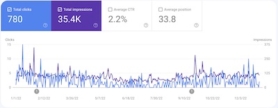The plot (click to embiggen) shows the number of times we appeared in a Google search (purple line, right-hand vertical axis) and the number of times there was a click through (blue line, left-hand vertical axis).

We have a pretty low click-through rate of 2.2%, which means as far as Google searchers are concerned, this really is a crummy little blog that nobody reads. Also, our rank in Google searches averages to about 33, i.e., on the 2nd page of hits where practically nobody ever looks. And I’m still ok with that.

As with last year, most of the clicks were from the Anglosphere, plus a long tail of everywhere else. Where are my French former colleagues?!

By device, there were about 3.75x more desktops than mobile, and just a couple of tablets. While technically this CLBTNR obeys the “rules” of being mobile-friendly, it sure looks better on a bigger screen.

Search queries

The top 2 queries – the only ones to make it out of single digits – were “yle editrix” and “ratio of two beta distributions”.

• The first is, as with last year, a mashup of “Your Local Epidemiologist” and “Weekend Editrix”, weirdly enough.
• The second points to the most technical page so far on this CLBTNR, and probably the only real research result that I’ve invented in retirement.

Well, at least one of them makes sense this year!

Linked pages, link text, and link text

The outside link report is largely unchanged from last year: most places link to the front page of the blog, unsurprisingly. The sources of those links are about the same, too: places in the comments sections of other blogs where I’ve dropped a pointer.

The Weekend Conclusion

Conclusion:

• Ok, it’s not like nobody reads this blog. There are a few readers, small in number but deeply crazed. Sort of like me.
• Google search hits are more or less useless, with a low click-through rate based on people looking for internet-famous personalities and some other random junk.
• Most readers are in the Anglosphere, and use desktops or laptops, a few phones and almost no tablets. I’m vaguely disappointed to have so few French readers.
• Linkage comes mostly from places where I’ve left comments and gotten (very minor) notice.

All in all, not that much change (other than messed-up comments which my messed-up brain has not yet fixed).

Thanks to my readers, all 6 or so of you!

Notes & References

1: WeekendEditor, “R script to analyze post statistics”, Some WeekendReading blog, 2023-01-01. Extensively revised for 2022. ↩

2: WeekendEditor, transcript and spreadsheet for all posts mid-2020 through year-end 2022, Some WeekendReading blog, 2023-01-01. ↩