
US Partisanship and Social/Economic Outcomes Revisited
Tagged:MathInTheNews
/
Politics
/
Statistics
For any US members of the Nerd Tribe who are a bit undecided on the relative benefits and harms of voting in the upcoming elections, let’s take another look at whether partisan control of the 3 branches of the US government makes any difference to economic and social outcomes. Summary: Republican presidents are bad & Democratic presidents are good for the deficit as a fraction of GDP. The rest mostly doesn’t survive LASSO regularization, leave-one-out crossvalidation, and a low error rate on predictions.
Conventional ‘Wisdom’
Let’s revisit the topic of whether Democratic/Republican control of the 3 branches of the US government affects economic and social welfare outcomes in each Congressional term. We’ve previously visited most of these these [1], and later remembered to include the US federal budget deficit. [2]
As we said last time, the motivation here is:
Conventional wisdom in the US is that Democrats are always better on social issues, but Republicans are always better on the economy & defense. I actually don’t quite know the basis for this. It’s probably just assuming that Republicans are either rich or in deep with big corporations, and thus should know a thing or two about making money.
However, as I vaguely recall economics Nobelist Paul Krugman saying, making money is one thing but managing an economy is quite another!
Mostly my memory of Republican rule since Reagan has been that they cut taxes only for the wealthy (which never “trickles down”), expand the military, start wars, restrict civil rights, and generally blow up the deficit and the national debt. If that memory is accurate – note the big “if” – then all of that can’t be good for the economy and the data should say so.
So let’s go find some data and see if we can interrogate it properly.
The Data and the Question
We’re going to look back about 50 years, to data starting in the congressional term of 1977-1978. That means there are 24 congressional terms from then until now, so we have really 24 data points. That’s not very many! We’d like, of course, to have more data. While we can go back further, there are a couple reasons not to do so:
- Some of the data series, like stock market returns of the index funds VFINX (S&P500) and VTSMX (US total stock market), and U6 (a broad measure of unemployment) don’t even make it back to 1977.
- Before 1977, you’re into President Ford (not elected, appointed for a partial term after Nixon) and then into Nixon and his predecessors. The US political world was very different then, with candidates largely chosen by party bosses, with only symbolic primaries. (Arguably, we’re already going back too far, since Reagan in 1980 was when the US Republican party started getting deeply crazy.)
So 1977 is about the limit of our visibility into a past which is both relevant and reasonably complete. And 2024, the final year of the Biden presidency, was the last congressional term for which we have complete data.
So that’s the 95th through the 118th congressional terms, in case you happen to be a Congress nerd. (I know there’s at least one among the readership of this Crummy Little Blog That Nobody Reads (CLBTNR). Yeah, I see you; you know who you are.)
The Partisanship Data
The partisan control data on the US House, Senate, and Presidency is widely available. I can almost do it from memory! However, to be totally on the up-&-up, we got the partisanship data from Wikipedia. [4]
It’s pretty straightforward, in the end: annotating each congressional term as Democrat or Republican, for the House, Senate, and Presidency.
An Exploratory Look at the Partisanship Data
We’d like to know if the 3 branches of the government tend to go together to a party, or if they’re relatively independent. We do this by:
- For each pair of branches (House/Senate, House/President, Senate/President), we make a 2x2 crosstabulation of Democrat and Republican counts.
- We assess the statistical significance of any row or column differences by both Pearson’s $\chi^2$ crosstabulation test and Fisher’s exact test, the latter being perhaps more appropriate for the small counts of our small dataset.
- If either of those come out statistically significant, we assess the strength of effect with Yule’s $\phi$ statistic.
 While we’d love to report some kind of relationship, look at the $p$-values reported for
significance in the table: nothing even vaguely approaches the traditional threshold of $p
\lt 0.05$. So we conclude that the $\phi$ statistic is meaningless here, and the 3
branches do not tend to switch parties in lockstep.
Thus we should expect trifectas (House/Senate/President all one party) to be rare.
The Social & Economic Outcome Data
We collected 9 different social and economic indicators, the detailed handling of which is explained in Appendix A:
- US inflation data is from the US Bureau of Labor Statistics, the CPI-U series for all urban consumers. [5]
- US unemployment rates, measured 2 ways, comes from the FRED database maintained by the
St Louis Federal Reserve.
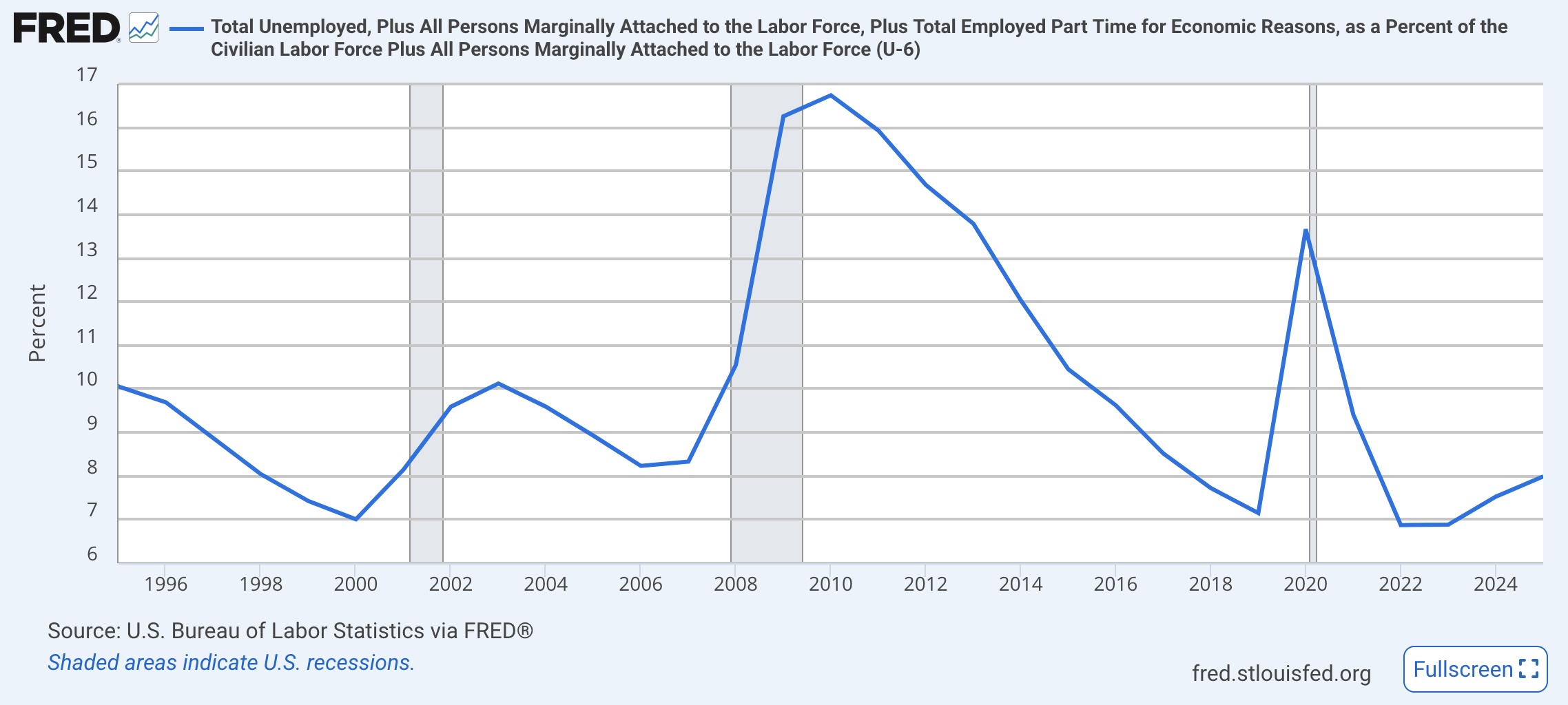
- We use a measure broader than the usual one, including ‘discouraged workers’ called U6. [6] This series goes back only to 1995.
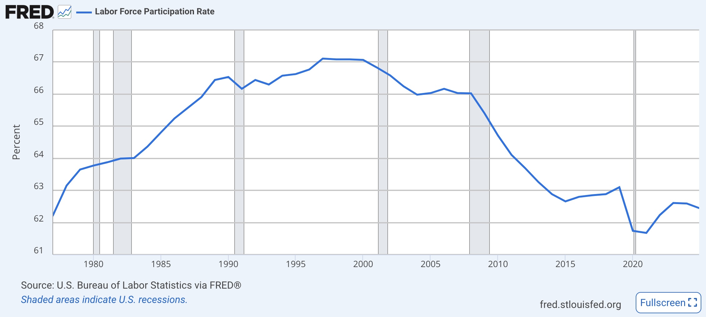
- We also use the labor force participation rate (LFPR), because it’s even harder to game. [7] This is harder to “game” than U3 or U6, e.g., by redefining “discouraged workers”. On the other hand, it has some baked-in demographics about the entry of women into the workforce, and the aging of the population as the Boomers age out. There’s not much we can do about that, short of building a regression model of LFPR on women as a % of workforce + mean workforce age, and using the residuals as a “corrected” LFPR. Perhaps another time!
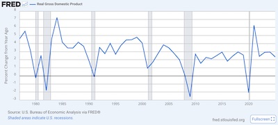
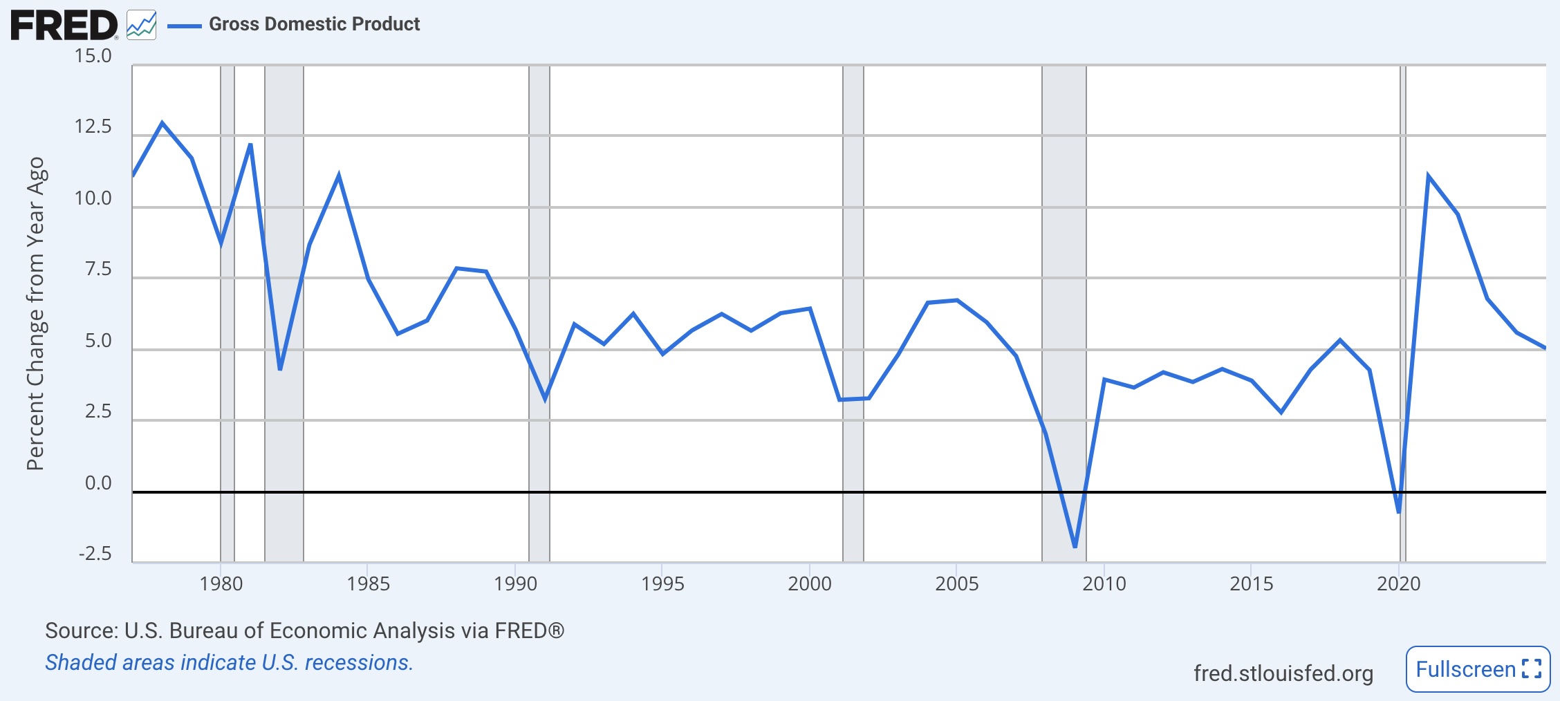
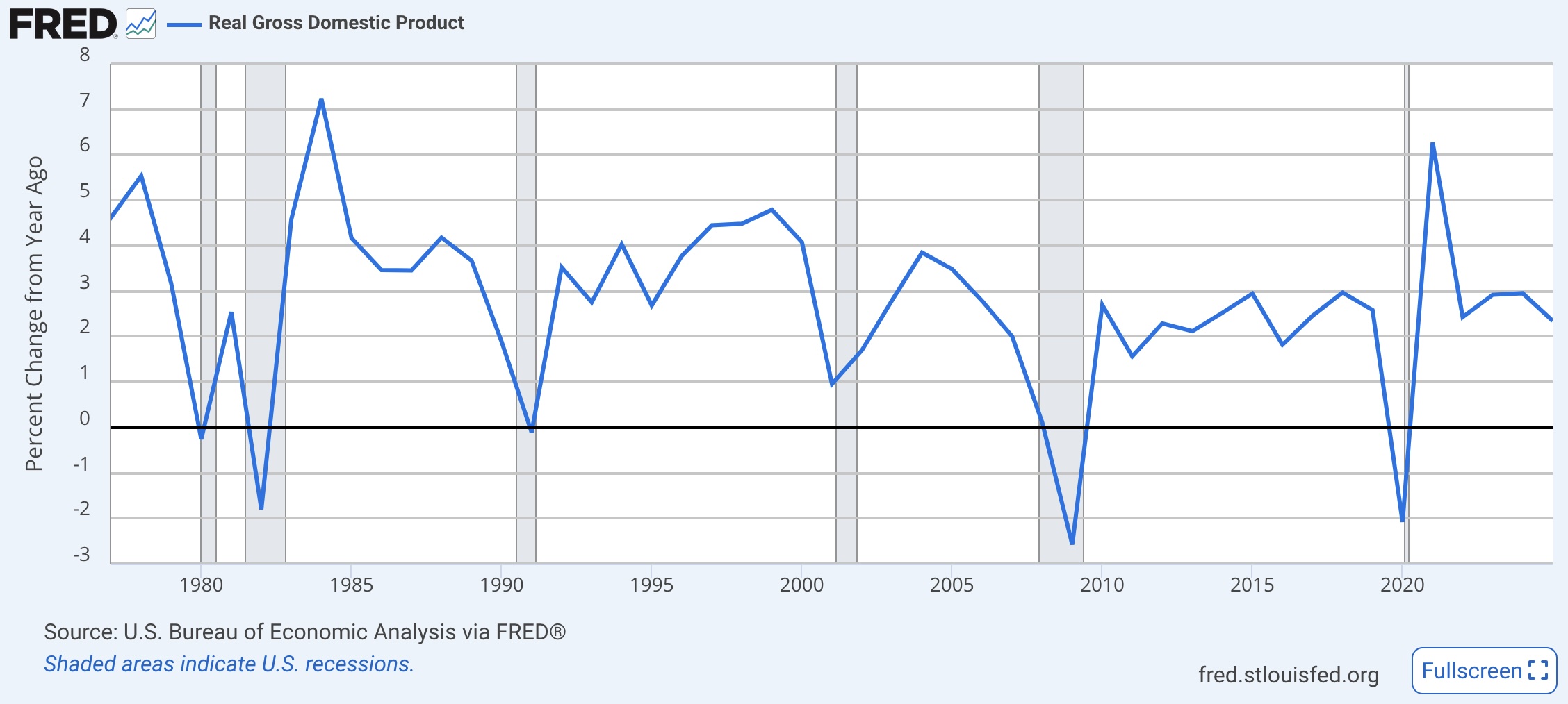
- The growth of the US economy we measure by Gross Domestic Product, again as reported by FRED at the St. Louis Fed. We use annual growth rates:
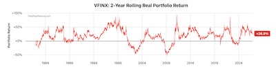
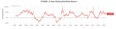
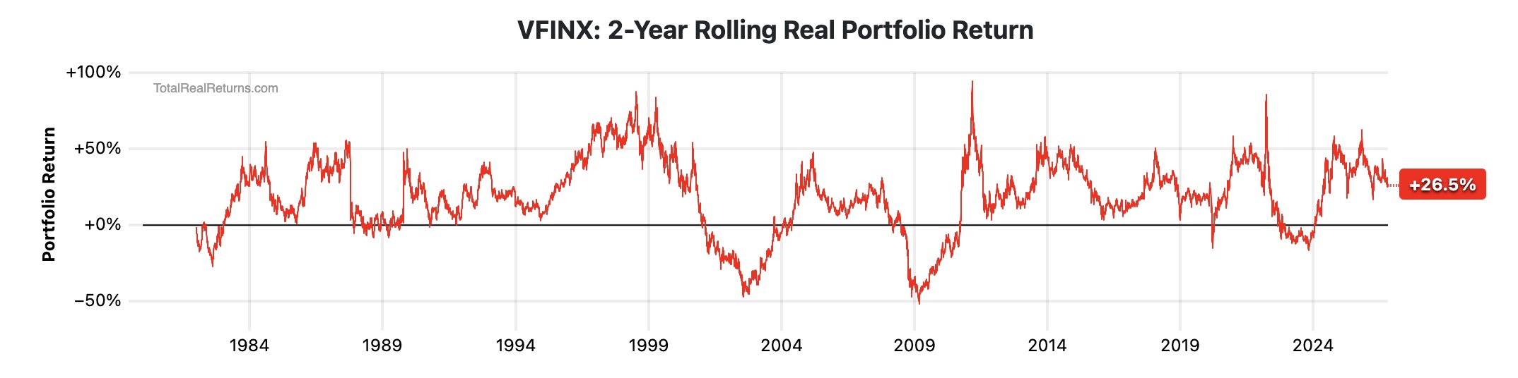
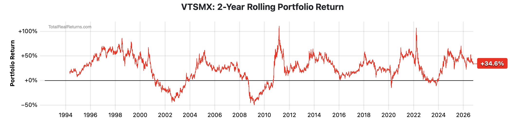
- US stock market returns, measured in real (inflation-corrected) terms, using actual index mutual funds in which consumers could have invested. These are historical returns, from funds actually in existence, not some calculation. We used the usual S&P500 index and the US total stock market index, which is a bit broader:
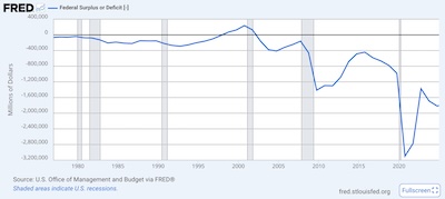
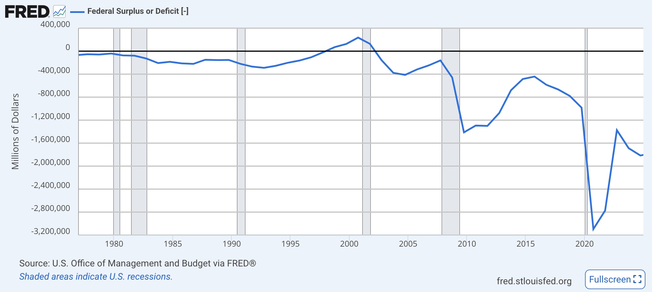
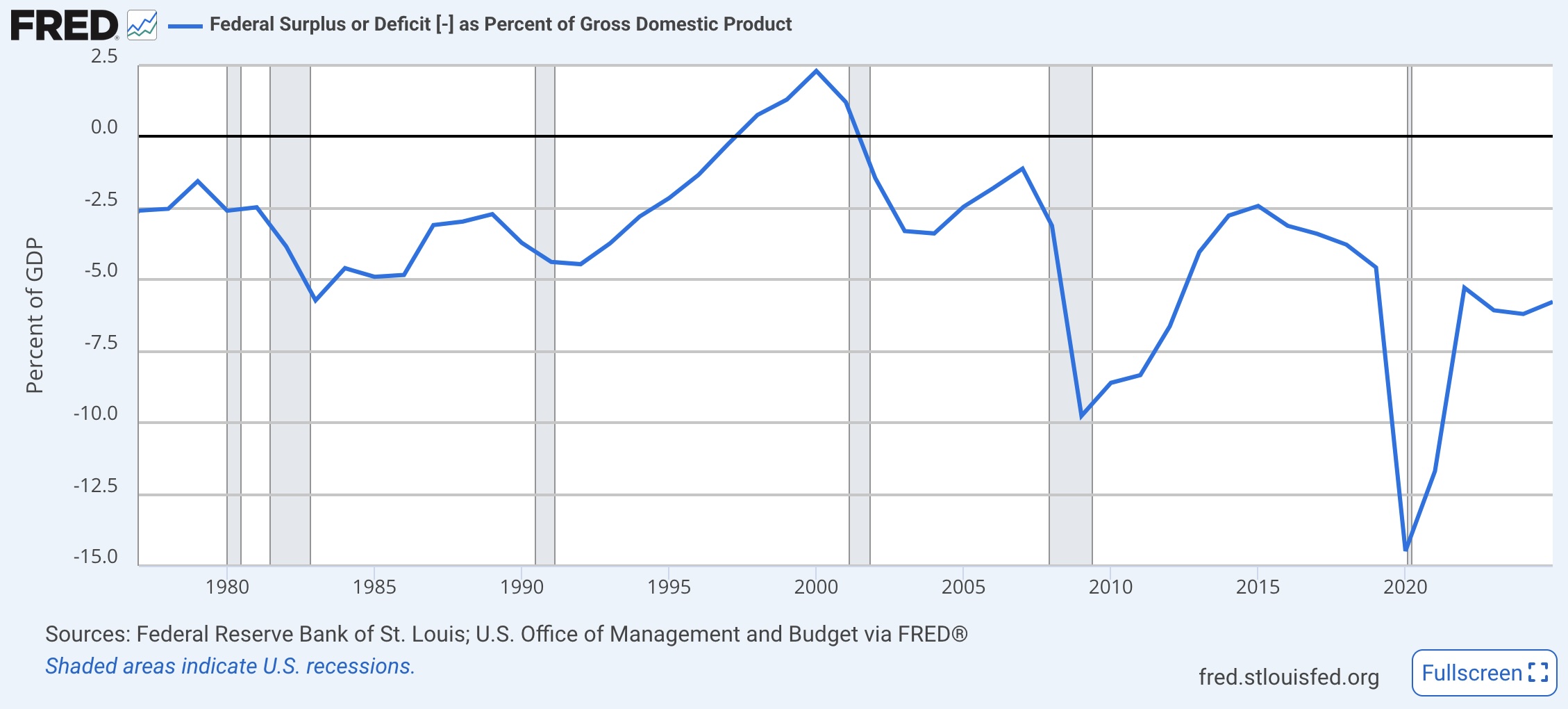
- The US budget deficit data again comes from FRED at the St Louis Fed:
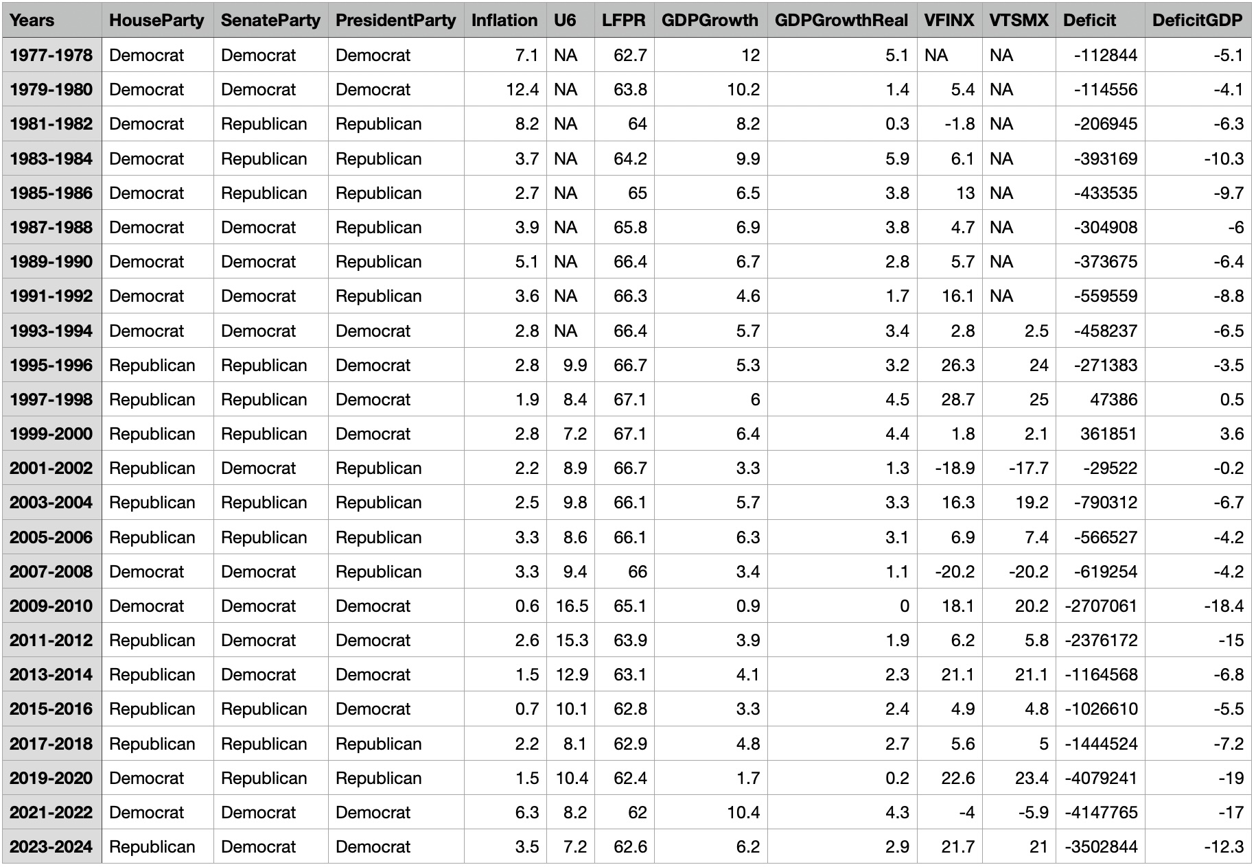 Processing that voluminous bolus of raw data as described in
Appendix A, we get our dataset, shown here in all its glory. Of
course, ‘all its glory’ is intended ironically: it’s only 24 rows, so we’re either
underpowered for doing anything very fancy or right on the edge of that.
(Shown here is the numerical version of the social & economic outcome data. What’s used in the regressions is the Good/Bad binarization as described above. This is more informative just for looking at by human beings.)
An Exploratory Look at the Social & Economic Output Data
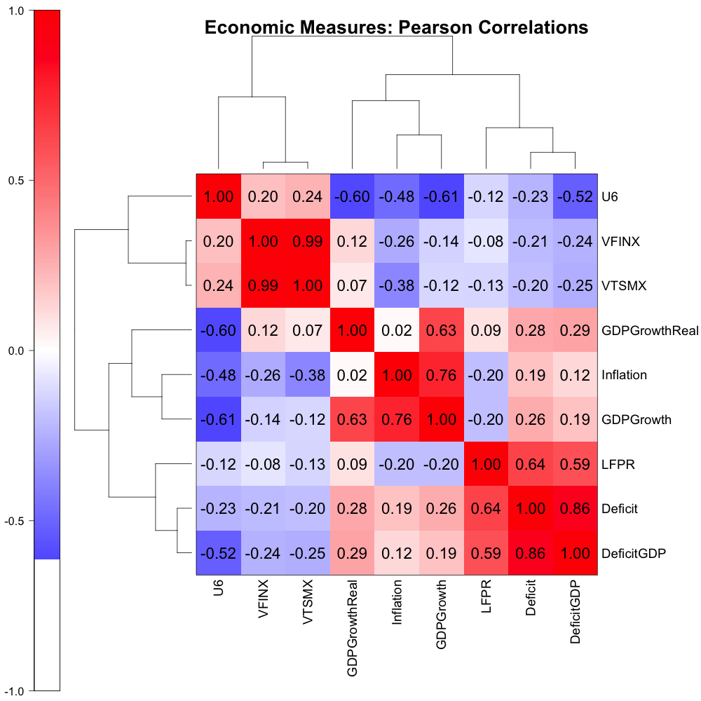 When faced with a matrix of continuous variables, variables on the columns and
measurements on the rows, every statistician will do the same thing: calculate a Pearson
correlation matrix, bicluster the result, and stare sagely at the pretty colors. (Your
better sort of statistician will first stare at the row and column dendrograms.)
And so it is here. (Click to embiggen!)
We used pairwise complete observations here, since some of the variables (VFINX, VTSMX, and U6) have some missing values.
As is always the case, the bicluster confirms some of our prejudices, confounds some others, and just presents some puzzles. Such is the fruit of the unsupervised learning tree:
- The dendrograms form 3 general groupings of U6/stock market, GDP/inflation, and deficit/LFPR.
- VFINX and VTSMX are basically the same thing (upper left corner). This makes sense, since both measure the US stock market.
- Considerably more puzzling is why the stock market is positively correlated with
unemployment U6. As we said last time:
I’d have thought higher unemployment would happen in recessions, when stock returns went low or negative.
Warren Buffet is supposed to have said “Bear markets are where you make all your money, you just don’t know it at the time.” I think he was talking about cost-averaging, i.e., your regular investments buy more shares in bear markets because the prices are lower, and in the long run that benefits you. Maybe not what’s happening here, though it came to mind.
Probably what’s happening here is the mild positive correlation is not statistically significant, given the paucity of our data.
- U6 is rather negatively correlated with GDP by both measures, and with inflation. (Blue block at center left and center top.) Recessions are more or less defined by decreasing GDP, and inflation & employment also tend to go down.
- I’d expected U6 and LFPR to be negatively correlated, but it appears that’s not by very much.
- GDP, real GDP, and inflation are all correlated. One can certainly understand the 2 GDP variables, but inflation probably creeps in because it happens during booms and inflates the currency that measures GDP.
The Question: Is There A Reasonable Prediction Model?
We then binarize the social & economic outcomes data from continuous variables to “Good” vs “Bad”. The detailed rules for this are described in Appendix A, but generally we ask things like whether inflation is above or below the Fed’s 3% target, whether GDP went up or down compared to the previous term, whether the budget is in deficit or surplus, and so on.
So all the social outcomes are binary coded.
We code the partisanship data a bit more interestingly, since we also want to consider doubles (same party in House/Senate, or House/Presidency, or Senate/Presidency), as well as trifectas (same party in all of House/Senate/Presidency). We avoid traditional dummy coding, in favor of basically measuring the number of branches controlled by a party. We score Republicans as +1 and Democrats as -1. The pairwise and triple predictors just sum those up:
- House, Senate, and President are coded as +1 for Republicans and -1 for Democrats.
- House+Senate, House+President, and Senate+President are coded as +2 if Republicans control both, 0 for mixed results, and -2 if Democrats control both.
- The triple combination, House+Senate+President, is scored +3 if Republicans control all, +1 if Republicans control two but Democrats have one, -1 if Republicans have one and Democrats have two, and as -3 if Democrats control all 3.
Armed with scoring for partisan control of branches separately and in combination, and binarized social outcome variables, we attempt a supervised learning model with logistic regression. That is, for each social/economic outcome variable, we try to predict the log odds ratio of it coming out as “Good” as a linear function of the partisanships:
\[\begin{align*} \log{\frac{\Pr(\mbox{Good})}{\Pr(\mbox{Bad})}} &= \beta_1 \mbox{HouseParty} + \beta_2 \mbox{SenateParty} + \beta_3 \mbox{PresidentParty} \\ &+ \beta_4 \mbox{HouseSenateParty} + \beta_5 \mbox{HousePresidentParty} + \beta_6 \mbox{SenatePresidentParty} \\ &+ \beta_7 \mbox{HouseSenatePresidentParty} \\ &+ \alpha \end{align*}\]Now, readers of this CLBTNR are a suspicious lot. (And I respect that!) You should be
squirming uncomfortably at my attempt to fit an 8-parameter model (the $\beta_i$’s and $\alpha$)
with only 24 data points! Fear not, for we fit using the
R glmnet package:
- We do leave-one-out crossvalidation (LOOCV) to estimate on a fairly objective level how the model is performing, in terms of the misclassification rate, i.e., how often it predicts Good/Bad incorrectly.
- We use LASSO ($L^1$ regularization) to select which variables to include in the regression, the optimal set being determined by crossvalidation.
Finally, a practical test: we use the model trained here to make predictions on the training data itself. Then we sort that by probabilities, and report a Mann-Whitney test of whether Good/Bad are enriched for the top & bottom of the list. That is, does this probabilistic model tend to sort the outcomes the way they actually came out?
Results
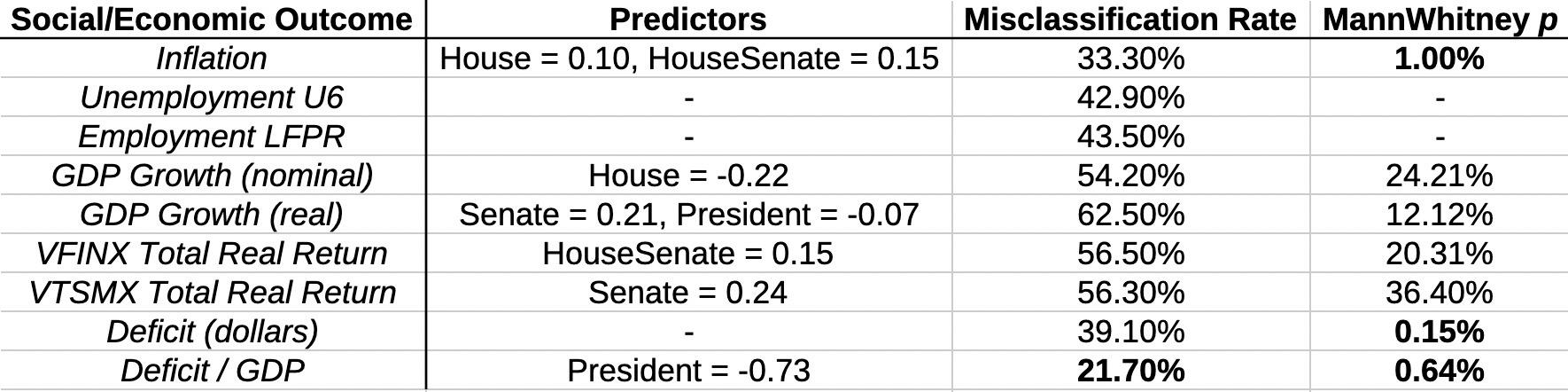 The table here shows the results of the regressions on each of the 9 social & economic
variables.
- If the 3rd column is blank, that means LASSO regularization has thrown out all the
partisan predictor variables.
- We should therefore conclude there’s no evidence of predictability from party politics in U6 unemployment, the labor force participation rate, or the deficit as measured in raw dollars.
- We generally want to demand a good $p$-value on the Mann-Whitney test, i.e., $p \lt 0.05$
to support statistically significant belief that the model’s predictions matter.
- On that basis, only inflation, and the deficit as a fraction of GDP matter.
- Finally, we’d like to demand a low misclassification error rate.
- The inflation prediction is pretty marginal, being wrong about 1/3 of the time!
- The prediction of the deficit as a fraction of the GDP, though, is only wrong about 1 time in 5.
So we conclude that the most believable result in terms of significance, which makes only moderate misclassifications, is the deficit as a fraction of the GDP:
\[\log{\frac{\Pr(\mbox{Deficit/GDP Good})}{\Pr(\mbox{Deficit/GDP Bad})}} = -0.73\times\mbox{PresidentParty} + 0.53\]where we’ve taken the value of $\alpha$ from the transcript.
The regression coefficient of -0.73 is the largest seen, and is negative. If you recall how we coded the partisan variables, negative regression coefficients favor Democrats and disfavor Republicans.
That is, contrary to the folk wisdom that circulates every election year, a Democratic president has been better for the deficit than a Republican president.
Most of the other stuff is harder to believe: it may survive regression, but with small coefficients, lousy Mann-Whitney performance, and high misclassification error rates. But deficit as a fraction of the GDP, we definitely must award to Democratic presidents.
The Peer Review Corner
Details on the data sources and their summarization are in Appendix A below. Details on the math of the prediction model, its regularization, & crossvalidation are in Appendix B below.
For your peer review pleasure, all of the materials necessary to reproduce this analysis are available below [3], including raw data (or as close as feasible), R scripts, a complete transcript of running those scripts, and all the result files thereby generated.
Paralipomenon, or Things Left Out
Probably lots of things could be done better! The ones I can think of:
- Data availability: I should probably have tried U3 in addition to U6, since it is available over more years. Similarly, I should have extended back the returns of VTSMX by using the Bogleheads historical asset returns spreadsheet.
- Sensitivity analysis: Could it be that this analysis is driven by a couple outlier datapoints? Could removing those outliers remove our conclusion about Democratic presidents, or summon from the void a result about Republicans? I don’t think so, and our use of cross-validation generally supports this. But a sensitivity analysis would be more specific about this.
- Time series: We’ve only looked at things that happen in a single 2-year congressional term, or a change from the immediate prior term. But often economic and social variables take years to react, and we’d only see that if we did a time series analysis on several prior terms, like an ARMA($n$, $k$) time series analysis. Alas, we have nowhere near enough data to be powered for that!
The Weekend Conclusion
Of the 9 social and economic outcomes we considered, only the deficit as a fraction of GDP survived, being better under Democratic presidents, worse under Republicans, and ignoring the other branches.
Other regressions either threw out all the political predictors via LASSO regularization, or had really small regression coefficients, or didn’t have good predictive power as measured by Mann-Whitney rank testing, or had high misclassification error rates that render them useless.
But in general, Democratic presidents are good.
(Ceterum censeo, Trump incarceranda est!)
(Et ceterum censeo, index Epsteiniani divulganda est!)
Appendix A: The Data
The data sources from which the data can be downloaded are in the references below. Also in Reference 3, is a link to the raw data as it was downloaded, for your comparison pleasure. Here are (most of) the details of how those raw data files resulted

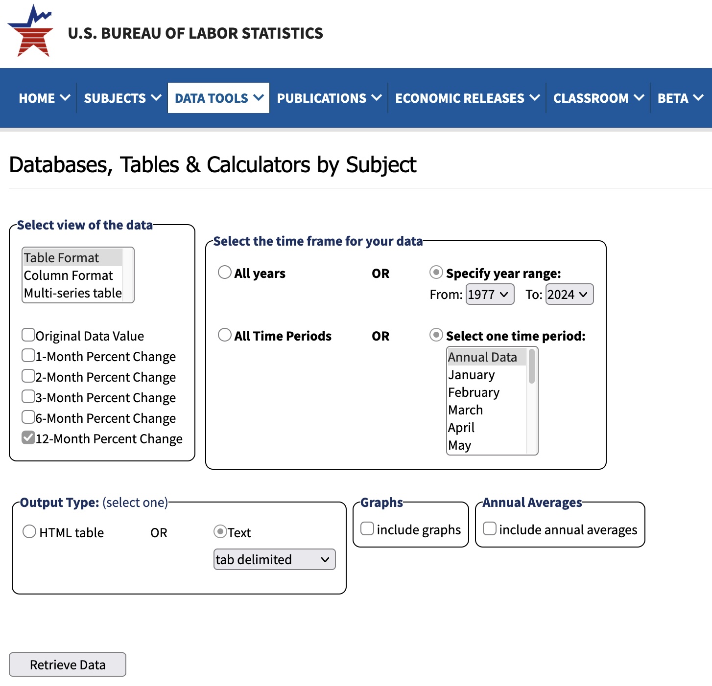
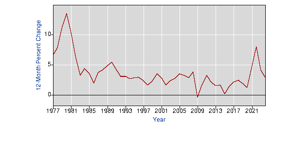
- Inflation, using the Bureau of Labor Statistics web page:
- Downloading: Obtaining the data, generating the datafile
bls-cpiu.tsv:- Choose CPI-U, for all urban consumers, from the series normalized to 1967 = 100.
- Choose “More formatting options.
- On the left-hand side, click “Select view of the data”. Choose “Table Format”, and then “12-month percent change”.
- On the right-hand side, choose 1977 - 2024. Then choose time period “Annual Data”. Then choose output type: “text, tab-delimited”.
- Combining: Since these are annual rates and congressional terms are 2 years, we combined inflation rates for the 2 years of a term using compounding: $(1 + r)^2 = (1 + r_1) \times (1 + r_2)$, with suitable additions and subtractions of 100% since these are given as percentages.
- Binarizing:
- The script has an argument for the Fed’s inflation target, defaulting to 3%. Inflation gets coded as “Good” if it’s at or below that level, “Bad” if above.
- Fed inflation targets have varied over the years, and indeed for some years there
probably even wasn’t one. So this is a bit of a simplifying assumption.
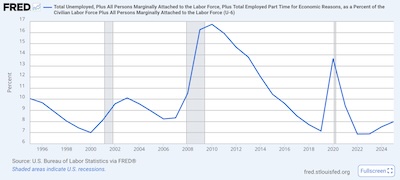
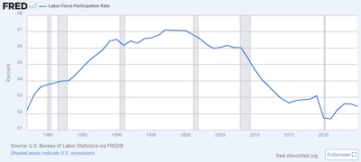
- Downloading: Obtaining the data, generating the datafile
-
Unemployment/employment rates, using the St Louis Fed’s FRED databases:
There are a lot of measures of unemployment! This is a fraction, with people looking for work in the numerator and total people available for work in the denominator. There is a lot of nuance in choices surrounding who counts for both of those sets. Men/women, prime working age 18-54, geographical regions, etc.
Most interestingly, the usually-reported measure of unemployment (called U3) does not include “discouraged workers”. To me this always smacks of human sacrifice: why do those people “not count”? So we choose the broader measures U6 and the Labor Force Participation Rate (LFPR).
- Downloading:
- U6: mysteriously only available from 1994 - date; I have no idea why. Choose
1995-2024, since those are the starts of congressional terms. Choose annual
percentages. NB that the file is comma-separated, not tab-separated. This generates
the data file
U6RATE.csv. - LFPR: Choose date range 1977-Jan-01 to 2024-Dec-31, and annual percentages. Also
comma-separated. This generates the file
CIVPART.csv(“civilian participation”).
- U6: mysteriously only available from 1994 - date; I have no idea why. Choose
1995-2024, since those are the starts of congressional terms. Choose annual
percentages. NB that the file is comma-separated, not tab-separated. This generates
the data file
- Combining: These are percentages, but they do not compound like inflation. We simply average over the 2 years of a congressional term to get a termwise value for U6 and one for LFPR.
- Binarizing: To rate the employment situation as good or bad, we take the first
differences of each series using the
diff()function in R. The first term gets an NA. After that U6 is “Good” if it went down or stayed the same “Bad” if it went up. LFPR does the opposite: “Good” if it went up, “Bad if it went down.
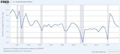
- Downloading:
- Economic growth, using the St Louis Fed’s FRED databases:
- Downloading: The two series we want are GDP PC1 (nominal GDP) and GDPPC1 PC1 (real GDP). Set the dates to 1977-Jan-01 to 2024-Dec-31. Select percent change from year ago, annual frequency, and aggregation method average. (The last shouln’t matter at the annual level, but I don’t quite understand it.) This is also comma-separated.
- Combining: Since these are growth rates, we combine them like inflation, using compounding, to get a 2-year figure for a congressional term.
- Binarizing: We rated a GDP growth rate as “Good” if it was at or above the median for
the dataset, and “Bad” if it was below.
-
Stock market real total returns
Rather than just use some stock index or other, we wanted a measure that was (a) actually investable by people of ordinary means, i.e., a mutual fund or ETF, and (b) included reinvestment of dividends and capital gains, and was corrected for inflation. So many times people report just the Dow Jones Industrial Average (itself a pretty nonsensical index), and forget about reinvestment and inflation.
So we used 2 different measures, each a retail index fund from Vanguard. They tend to be replaced by other “Admiral” versions nowadays, but they have a long tail into history that’s useful for our purposes.
-
Downloading: We used the Total Real Returns web site in the references, and set the start date to 1977-Jan-01. Turn on inflation adjustments and reinvest dividends. (One assumes this includes other distributions, like capital gains? But it was unclear.)
So we downloaded the files, added Year and ticker name as column titles. WE changed space-tab occurrences to just a tab. We removed the % signs. We changed their funky Unicode + and - signs (why do people do that?!) to plain old ASCII + and - signs.
VFINX starts in 1979 (also the start of a congressional term), so we recorded NA in 1977 and 1978. VTSMX starts in 1992, so we started recording in 1993 at the start of a congressional term and put in NA’s before that.
- Combining: Like inflation, these are percentage rates that combine with compounding, so that’s what we did to get a compound total real return across the 2 years of a congressional term.
- Binarizing: Like GDP and real GDP, we rated a stock market return as “Good” if it was
at or above the dataset median, and “Bad” if it was below.
-
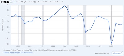
- Federal budget deficit, using the by-now familiar St Louis Fed’s FRED databases.
- Downloading:
- Absolute: Using the data series FYFSD, we got data for 1977-Jan-01 through 2024-Dec-31. The units are millions of dollars. The time points are Sept 30 of each year, ie., the end of the federal fiscal year. We took that value as representative for the whole year.
- As a fraction of GDP: We took the series FYFSGDA188S, using data from 1977-Jan-01 through 2024-Dec-31. It’s a dimensionless fraction of GDP, and the dates are on Jan 01.
- Combining: We just summed the deficit values over the years of a congressional term. (That’s not quite right if the GDP grew significantly during the term, but pretty close.)
- Binarizing: Again by taking first differences, we scored a deficit reading as “Good” if it increased from the previous term (recall deficits are negative, so an increase is a move up toward 0, or balance!), otherwise “Bad”.
- Downloading:
That’s quite a lot of work, but the R scripts pretty much automate most of it.
Appendix B: The Regression Method
 Of course we used the venerable R package
glmnet,
which is more or less the standard place to go for regression with crossvalidation and
regularization by LASSO, ridge, or elastic net. Indeed the package name is a shortening
of “generalized linear models with elastic net”. There’s a lot written about it, and
formidable statistical learning theory books about the method. However, a recent web
publication by the authors (soon to appear in print?) [14]
seems to be a good practical guide.
If you are already somewhat familiar with the statistics and want to learn about how to
use glmnet to reproduce this analysis, the relevant sections are
1-6 (general introduction to regularized regression and crossvalidation),
and
7 (binary classification, with emphasis on logistic regression).
We do not propose to write our own tutorial here, tempting as it is. We merely note that our choices were:
- Use logistic regression, on the “coded” partisan variables as above.
- Do leave-one-out crossvalidation, on recommendation of the package authors (which came
as news to us):
In our extensive simulations, we have found that as $K$ increases, the bias in CV error decreases significantly, while the variance does not increase much. As such, we recommend using LOOCV in situations where run time is not an issue. For all other cases, we recommend using industry norms $K$ = 5 or $K$ =10.
Since, according to the transcript, our analysis took about 1 sec total, we decided to take their advice as computing time was certainly not an issue! - We elected LASSO regularization, i.e., a penalty for each nonzero regression coefficient that made the algorithm “squeeze” to find just the optimal set of predictors.
-
The measure we optimized on was the misclassification rate, i.e., how often the resulting regression model incorrectly predicted a “Good” or “Bad” outcome. This is as was advised in section 7.2.3 in the reference above. The model used crossvalidation to determine how hard to squeeze, and we chose the best model (i.e., $\lambda_{\mbox{min}}$).
The results .zip file, available in reference 3 below, has all the relevant plots of misclassification rate versus number of parameters. They’re kind of ugly, since misclassification is by its nature a discrete integer number of mistakes out of 24 chances in our 24-sample dataset.
Notes & References
1: Weekend Editor, “US Political Parties and the Economy”, Some Weekend Reading blog, 2024-Oct-28. ↩
2: Weekend Editor, “US Political Parties and the Budget Deficit”, Some Weekend Reading blog, 2024-Dec-05. ↩
3: Weekend Editor, “Transcript of analysis of US partisanship and social/economic outcome data”, Some Weekend Reading blog, 2026-Oct-30.
In addition to the transcript which records all results printed during this analysis, we also make available for your peer review pleasure:
- A
.zipfile of the raw data as downloaded from the sources in these references, with as little manual manipulation as we could reasonably do. - A
.zipfile of all the scripts, written in R, for performing this analysis. This is everything you need to redo these computations, assuming you can install from CRAN the widely used R librariesplyr,vcd, andglmnet. - A
.zipfile of all the raw result files generated by these computations. - A Libre Office spreadsheet of the omnibus data shown in the image above. If you want to peer review just the regression analysis, you probably should start here.
Armed with the transcript and those downloads, you can decide both whether we’ve honestly reported the results here, and form your own opinion about our choices of datasets, analysis methods, implementation of them, and our interpretation of the results. ↩
4: Wikipedia Editors, “Party Divisions of the United States Congress”, Wikipedia, downloaded 2026-Oct-20.
This links to a table of the partisanship of the 3 branches of US government. We kept the part from 1977 (Carter) through 2025 (Biden), keeping only some of the more relevant columns.
- Alas, the majority in control was denoted by color, so (obligatory glare in statistician: grrr!) we explicitly tabulated that.
- The congressional terms were denoted something like 1977 - 1979, left-inclusive and right-_exclusive_. Oh, c’mon! We hand-edited the data to denote a 2-year congressional term by the years it held power, e.g., 1977-1978. You know, like normal people. (No, I’m not normal. But I can sometimes simulate it, to a degree, when required. But only when required.)
- The dash character used in the congressional terms was a weird Unicode emdash character, 0x2013. We manually changed it to a dash character. You know, like normal people.
- In 2001 during the Lesser Bush administration, the Senate was 50-50 so Vice President
Cheney would cast the deciding vote for Republican control. Sen Jeffords then changed
parties, Republican to Democratic. So in this term, Republicans had Senate control for
a few months, but almost all the term was in Democratic control. So we annotated this
as Democratic. There were other changes of party, but none of them shifted majority
control.
↩
5: US Bureau of Labor Statistics, “Consumer Price Index, All Urban Consumers (CPI-U)”, US BLS web site, downloaded 2026-Oct-21.
This is the annual percent change, using the series normalized to be 100 in 1967. ↩
6: St Louis Federal Reserve Bank Staff, “U6 Unemployment Time Series”, BLS via St Louis Federal Reserve Bank FRED system, downloaded 2026-Oct-22. ↩
7: St Louis Federal Reserve Bank Staff, “Labor Force Participation Rate Time Series”, BLS via St Louis Federal Reserve Bank FRED system, downloaded 2026-Oct-22. ↩
8: St Louis Federal Reserve Bank Staff, “Gross Domestic Product Time Series”, BLS via St Louis Federal Reserve Bank FRED system, downloaded 2026-Oct-22. NB: This is nominal growth, not corrected for inflation. ↩
9: St Louis Federal Reserve Bank Staff, “Real Gross Domestic Product Time Series”, BLS via St Louis Federal Reserve Bank FRED system, downloaded 2026-Oct-22. NB: This is real growth, after correcting for inflation. ↩
10: TotalRealReturns Staff, “VFINX Total Real Return Time Series”, TotalRealReturns.com web site, downloaded 2026-Oct-22.
NB: The returns used here turned on both distribution reinvestments and inflation correction to get a total, real return series.↩
11: TotalRealReturns Staff, “VTSMX Total Real Return Time Series”, TotalRealReturns.com web site, downloaded 2026-Oct-22.
NB: The returns used here turned on both distribution reinvestments and inflation correction to get a total, real return series.↩
12: St. Louis Fed Staff, “Federal Surplus or Deficit (FYFSD)”, FRED databases, US Federal Reserve Bank of St Louis, data from 1977 – 2024 retrieved 2026-Oct-22. ↩
13: St. Louis Fed Staff, “Federal Surplus or Deficit - as Percent of Gross Domestic Product (FYFSGDA188S)”, FRED databases, US Federal Reserve Bank of St Louis, data from 1977 – 2024 retrieved 2026-Oct-22. A local copy is archived here for peer review purposes. ↩
14: K Tay, E Craig, B Narasimhan, R Tibshirani, and T Hastie, “glmnet is (almost) all you need”, downloaded 2026-Oct-20, to appear in print. ↩
Gestae Commentaria
Comments for this post are closed pending repair of the comment system, but the Email/Twitter/Mastodon icons at page-top always work.