Election Night of the Living Beta Binomials

As you may have heard, the US is about to face an election more contentious than any since the Civil War. With vote counting likely drawn out due to right-wing mischief at, for example, the Post Office, what are we to make of partial returns as far as predicting the outcome? And will there be zombies?

The problem

Imagine we lived in a simplified, and and much more desireable, world:

• There are only 2 candidates for election, hereinafter termed GoodGuy and BadGuy. (US politics is downright Manichaean at the moment.)
• There is no Electoral College; rather the election is decided by direct popular vote.
• There is no red mirage/blue shift effect (in-person votes preferred by one party are known on election night, but mail-in ballots preferred by the other get counted more slowly over the next couple days).
• The number of popular votes to be cast, $N$, is somehow known in advance.
• The candidate accruing $K \geq \left\lceil N/2 \right\rceil$ votes wins. Since there are only 2 candidates and all $N$ ballots always vote either GoodGuy or BadGuy, this will surely happen one way or the other.

So here we are on election night, anxiously listening to the returns (on NPR or PBS, of course, since we’re GoodGuys — though the BBC and the Guardian get honorable mention). Out of $N$ ballots to be counted, just $n < N$ have been counted so far. They add up to $k < n$ votes for GoodGuy.

What should we predict about the final outcome from this partial information?

• In particular, what is the probability distribution $\Pr(K | N, n, k)$ for the final number of GoodGuy votes?
• What is the probability $\Pr(K \geq \left\lceil N/2 \right\rceil | N, n, k)$ for a GoodGuy win, i.e., the cumulative distribution function?
• Will the media ever learn this, and report accordingly?

With the exception of the last question, for which the answer is apparently and unfortunately a hard “no”, the other questions can be addressed probabilistically.

The model

Meet your new best friend, the beta-binomial distribution, which, as from its name ^[1], combines features from:

• the binomial distribution (probability distribution of votes for GoodGuy out of $n$ voters, each with probability $p$ of voting GoodGuy), and
• the Beta distribution (probability distribution for $p$, based on already observed voters in the same population).

If we somehow knew the probability $p$ of individuals voting GoodGuy, then the total GoodGuy votes would be binomially distributed:

But we don’t know $p$. We do have a sample of $n$ votes, $k$ of them for GoodGuy. A frequentist might plug in the point estimate $p = k/n$ and be done with it. That’s not bad, but we can do better: we can use Bayesian methods to get a posterior distribution for $p$, thereby capturing our knowledge gleaned from $(n, k)$ observations, and our remaining uncertainty.

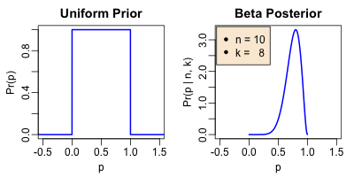
Let’s start with a uniform prior on $p$, i.e., we are maximally ignorant and believe any value in $[0, 1]$ is as likely as any other:

where $\theta()$ is the Heaviside step function, here ensuring that $p$ has support only in $[0, 1]$.

The likelihood function for $p$ when we observed $k$ out of $n$ votes is binomial

Mash them together in Bayes’ rule, and note that the result is a beta distribution:

where $B(k+1, n-k+1)$ is the normalization integral, our old college buddy from freshman year, the complete beta function. This distribution is a beta distribution of the first kind, with the parameters in the usual notation being $\alpha = k+1$ and $\beta = n-k+1$. ^{[2] [3]} The figure illustrates an example with $n = 10$ and $k = 8$, e.g., if you flip a coin 10 times and it comes up heads 8 times, what should you believe about the probability $p$ of flipping heads?

The beta-binomial distribution combines these: pick a value for $p$ from a beta distribution, then draw binomial samples using that $p$. It just wraps all of that process up into a single distribution function:

where we’ve conveniently written everything in terms of the complete beta function.

The probability of a win is the cumulative distribution function,

That can be written in terms of the generalized hypergeometric function ${}_{3}F_{2}()$, but that’s likely more trouble than it’s worth. ^[4]

Parameter estimation

There are loads of papers, and implemented algorithms, for doing beta binomial parameter estimation (e.g., references 5-7). However, here we don’t actually have multiple samples from a beta binomial with which to work; we have one sample in the form of the two numbers $(n, k)$. So we pulled a swift one above: we chose the beta binomial parameters $\alpha$ and $\beta$ so that the binomial part of it best reflects the $(n, k)$ observed. This is sort of a poor man’s maximum likelihood.

Practical use

As with so many things when working in R, someone has beaten me to it: the TailRank package (reference 8) already implements the beta binomial distribution, its cumulative distribution, and many other things. That’s the nice thing about working in a language with a vibrant user community: other people largely write your software for you. (reference 9)

The US currently has a population of about 328 million. How many of those can be expected to vote? According to Wikipedia on US voter turnout in US presidential elections, about 40% – 42% in the recent past. A turnout of 45% of the population (a higher fraction of eligible voters) would be a new record. So let’s go with 45%.

Let’s suppose early returns have given us the results for 500,000 voters, and it’s 250,500 votes for GoodGuy (just a hair over half). What’s the chance of a GoodGuy win?

> probWin(N, n, 250500)
[1] 0.9209983

That’s odd… with a bare margin of 500 votes out of 500,000 — 1 in 1000! — we’re suddenly very confident of a win at 92% probability. How can that be?

…and why it’s not so practical

There are a number of infelicities in models like this. Among them are the 2 that are tricking us into over-confidence:

• The assumption that the early votes are entirely randomly selected, and in no way reflect underlying political structures, are not biased for one candidate, etc. This is, of course, false.
• The very large numbers here, where we’re looking at 147 million voters, and 500,000 early voters. As numbers like that get large, the statistical significance of a model zooms upward, generating more and more certain predictions. For reasons entangled with the first, this is, of course, false: you might have large numbers, but they’re biased large numbers. The red mirage/blue shift effect is a real thing, large cities with lots of liberal voters take longer to tabulate than small districts, and so on.

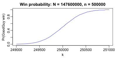
To illustrate this, consider the same problem above ($N$ = 45% of 328 million votes to be cast, $n$ = 500,000 already counted) but now vary the number of already counted GoodGuy votes $k$ from 249,000 to 251,000. This is clearly a very small variation. But note in the figure that the probability of a GoodGuy win goes from nearly 0 to nearly 1! Moving just 1000 votes either way makes the model swing wildly in its prediction. Over the course of election night, as the tallies vary, our predictions would swing wildly back and forth.

Conclusion: We’ve had a lot of fun here, and for nerdly types like your humble Weekend Editor this is a good anxiety relieving process. But we’ve modeled an over-simplified world. Our model has failed to be believably predictive.

The sad facts: There are more than 2 candidates in most jurisdictions, and thus a significant spoiler effect (Ralph Nader in 2000, anyone?). There is, sadly, an Electoral College and it severely biases voting in the US towards Republicans representing rural, sparsely populated, conservative districts. The backup for the Electoral College, voting in the House of Representatives, is also biased: each state gets 1 vote, again over-representing rural conservative states. The red mirage/blue shift is a real thing. The candidate elected seldom gets a majority (though some states are now experimenting with rank-preference voting mechanisms of various sorts, which would help). It’s important to enumerate your assumptions, as we did at the outset, so later you can see if they’ve steered you wrong.

So… hang on. There may yet be zombies.

Notes

1: As they say in Japan: “名は体を表す” (na wa tai o arawasu), or “names reveal the inner nature of things”. In equally pretentious Latin, nomen omen est. This is, of course, strictly false; but it is occasionally useful for pretending one knows whereof one speaks. ↩

2: In particular, a $B(1, 1)$ distribution is just the uniform distribution, so it’s betas all the way across the board. ↩

3: Binomial and beta are conjugate priors: if you observe $k$ out of $n$ binomially-distributed samples, then the beta distribution tells you what to believe about the underlying $p$ that generated those votes. Heckerman’s Bayesian tutorial (reference 4), for example, explores this in a tutorial way, with a coin-toss example to estimate how the coin is loaded.↩

4: Your humble Weekend Editor is still working through some childhood trauma around early exposure to hypergeometric functions. ↩

References

1. T Vladeck, “Unpacking the election results using bayesian inference”, TomVladeck.com, 2016-12-31.

2. E Kaplan & A Barnett, “A new approach to estimating the probability of winning the presidency”, Operations Research 51:1, 2003-Jan/Feb, 32-40.

3. “Beta-binomial distribution”, Wikipedia, last edited 2020-04-26.

4. D Heckerman, “A tutorial on learning with Bayesian networks”, Arxiv.org, 1996-Nov (revised 2020-Jan).

5. T Minka, “Estimating a Dirichlet distribution”, Microsoft Technical Report, 2000 (revised 2003, 2009, 2012).

6. RC Tripathi, et al., “Estimation of parameters in the beta binomial model”, Ann Inst Stat Math, 46:2 (1994), pp 317-331.

7. Y Qassim, A Abassi, “Parameter estimation of Polya Distribution”, unpublished talk.

8. K Coombes, “TailRank R package”, CRAN 2018-May-18.

9. Weekend Editor, night-of-the-living-beta-binomials.r, Some Weekend Reading, 2020-Aug-07.