On Close Elections

Closely contested elections are the cause of a lot of fighting among partisans. Let’s see what it would mean to have that fight in as objective, statistically principled manner as possible. We’ll use the currently still-contested Mississippi election for US Senator as an example.

The Mississippi Election for US Senator

One of the ways I react to stress is by over-analyzing things, just to be as certain as I can be that I haven’t overlooked anything. Today I’m worrying about the last couple Senate elections yet to be called.

Mississippi is, to put it mildly, a very red state. It is almost the archetype of southern US states: venomous racism in its history (and its present), fanatical conservative Republicans, endless voter suppression (with a history of actually murderous intimidation of Black voters), anti-education, and relatively poor.

It is therefore notable that this race, among 3 politicians, involves 1 White Republican woman 2 Black men (1 Democrat and 1 independent but former Democrat). This could be the first time Mississippi has elected a Black to the US Senate since Sen. Blanche Bruce in 1874, during the Reconstruction period after the American Civil War. (Indeed, the American failure to finish Reconstruction seems to be at the root of many of our problems with far-right racist politics today.)

Dramatis personae:

• Scott Colom, the Democratic candidate.

• Cindy Hyde-Smith, the Republican candidate and incumbent.

  Interestingly, Colom was nominated for a federal judgeship under Biden with the backing of enough Republicans. However, Hyde-Smith blocked the appointment by failing to return the “blue slip”, a Senate mechanism whereby senators can veto appointees from their state in an unreviewable and unchallengeable way. There may be some animus here about that!

• Ty Pinkins, a former Democrat who, having been eliminated in the primary, decided to run in the general as an independent. In a close contest, such a “spoiler” candidate can decide the race by siphoning off votes from one of the major candidates.

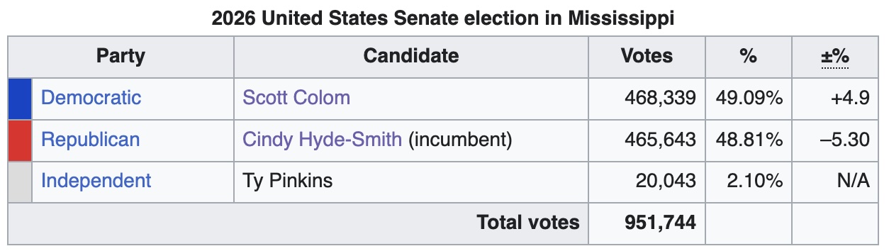Here’s the current state of vote counting, one week after election day, as reported in Wikipedia. ^[1] It appears that almost 97% of the expected votes have been tallied, so this would ordinarily be the endpoint.

• However, the margin between Colom and Hyde-Smith is razor-thin, at 2696 votes. If, as is claimed, “several thousand” absentee and provisional ballots remain to be counted (or not… remember, this is an era when Republicans are famous for vote suppression), then they could flip the election either way.
• Also, note that the vote count for Pinkins is about 7.5x larger than the spread between the major candidates. If he hadn’t run, this would all be over now. Whether the voters for Pinkins (a former Democrat) would have gone for the current Democrat is… unknowable, but that won’t stop pundits from talking about it as though they could know it.

So as of this moment, Colom holds a slim lead by 100% * 2,696 / 954,025 = 0.28% of the votes. If less than 2,696 absentee & provisional ballots remain to be tallied, then it’s mathematically impossible for anyone but Colom to win. (Barring a recount, á la the Florida 2000 presidential election, where hijinx ensue to discard or reassign ballots. Don’t rule out that Republicans might try that again!)

Statistics of a 3-Way Election

Here’s our model of how to think about an election: each of the $1,\ldots,C$ candidates has a certain probability $p_1,\ldots,p_C$ to attract the vote of any given voter. These are constrained by:

\[p_1 + \cdots + p_C = 1\]

because everybody who voted picked one of the candidates; the $p_i$’s represent probabilities assigned to disjoint outcomes, one of which always happens, i.e., a voter eventually chooses a candidate.

We would like to put in office whichever candidate has the largest $p_i$.

There are 2 problems:

• It might be that candidates $i$ and $j$ have very nearly equal $p_i$’s. Given the inevitable uncertainty surrounding estimating them, we have to have some rules around addressing ties. This is one reason I like ranked-choice voting, with its instant-runoff character. At the end of counting, somebody has a majority of either first choice or subsequent choice votes!

  (We have little else to say about this issue, for now.)

• More immediately, we do not know the values of $p_i$!

We can think of an election as an experiment (statistically: a multinomial trial), to collect observations that let us estimate $p_i$ to get both a value and some kind of uncertainty around it. (In a sane system, we’d have runoff elections if the top vote getters were all within the same margin of error. This is not that system.)

In the election, each candidate gets $n_1,\ldots,n_C$ votes. The total number of votes cast is $N = n_1 + \cdots + n_C$, not counting abstentions, write-ins, and all the usual craziness around the margins. This single experimental observation of the vector of integers $(n_1,\ldots,n_C)$ is all we get!

• A frequentist would estimate $p_i \approx n_i / N$ and be done with it. This amounts to just counting the votes and giving up on any uncertainty measurement. (Admittedly: there are some kinds of corrections our hypothetical frequentist can apply for small sample sizes, and ways to get some kind of uncertainty measurement in some cases.)

• A Bayesian would sigh resignedly upon hearing that.

  Instead, we should first state the probability model of accumulating votes to get $\Pr(n_1,\ldots,n_C | p_1,\ldots,p_C)$ and then invoke Bayes rule to get a distribution of values for the $p_i$’s, i.e., $\Pr(p_1,\ldots,p_C | n_1,\ldots,n_C)$.

We start with a simple model using a multinomial distribution:

\[\Pr(n_1,\ldots,n_C | p_1,\ldots,p_C) = \frac{N!}{n_1! \cdots n_C!} p_1^{n_1} \cdots p_C^{n_C}\]

This lets us compute the probability of the election outcome $(n_1,\ldots,n_C)$. Our frequentist sibling would appeal to Maximum Likelihood Estimation (MLE) by choosing $p_1,\ldots,p_C$ so as to maximize the probability of the election results we see. However, our hypothetical Bayesian would use Bayes’ Rule to derive the conjugate prior distribution for $p_1,\ldots,p_C$, the Dirichlet distribution, in our notation:

\[\Pr(p_1,\ldots,p_C | n_1,\ldots,n_C) = \frac{1}{B(n_1, \ldots, n_C)} p_1^{n_1+1} \cdots p_C^{n_C+1}\]

where

\[B(n_1, \ldots, n_C) = \frac{\Gamma(n_1 + 1) \cdots \Gamma(n_C + 1)}{\Gamma(n_1 + \cdots + n_C + C)}\]

is a multivariate generalization of the complete Beta function.

Note that in this notation, when all $n_i = 0$, the distribution on $p_i$’s is uniform, i.e., an uninformative prior before the election.

At that point, we usually follow the crowd and choose a MAP (maximum a-posteriori probability) estimator, which here amounts to choosing the mode. Uncertainty estimates come from various ways of measuring how wide the distribution is around the mode. The mode is pretty easy to compute:

\[\hat{p_i} = \frac{n_i}{N}\]

which is just what our frequentist might have chosen!

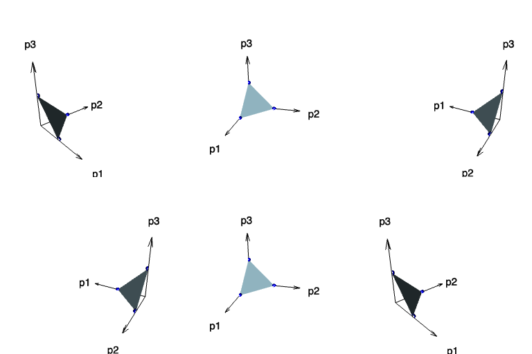Now consider the case $C = 3$, e.g., the 3 candidates we have in Mississippi. There are 3 probabilities $p_1$, $p_2$, and $p_3$, so it’s tempting to conclude we’re in a 3-dimensional space. But the constraint that they all have to add up to one means we get reduced back down to 2 dimensions. The additional constraint bounding $0 \le p_i \le 1$ means we are restricted to the surface of the triangle shown in this animation: a triangle that intersects each axis at 1.

That triangle is the manifold of 3 probabilities which all are constrained to add up to 1.

Somewhere in that triangle is the point we want. People don’t usually make a 3d plot like this and scribble on the triangle; they just draw the triangle with the constraint that coordinates along the edge all add up to 1. This is the ternary plot, well-known among those who care about such things. (I once had to deal professionally with the case of $C = 4$, in dose-optimizing a combination of 4 different mRNAs. Instead of a triangle, we had a tetrahedron of mixtures to consider. That was fun! Explaining it to the biologists was… well, an uphill climb for all of us.)

Here’s the result of computing the Dirichlet MAP estimator. Note that it’s pretty much identical with the naïve estimator of just taking the fraction of the total votes. It’s important to inspect such constraints, to make sure we haven’t committed some blunder that’s driven us off track!

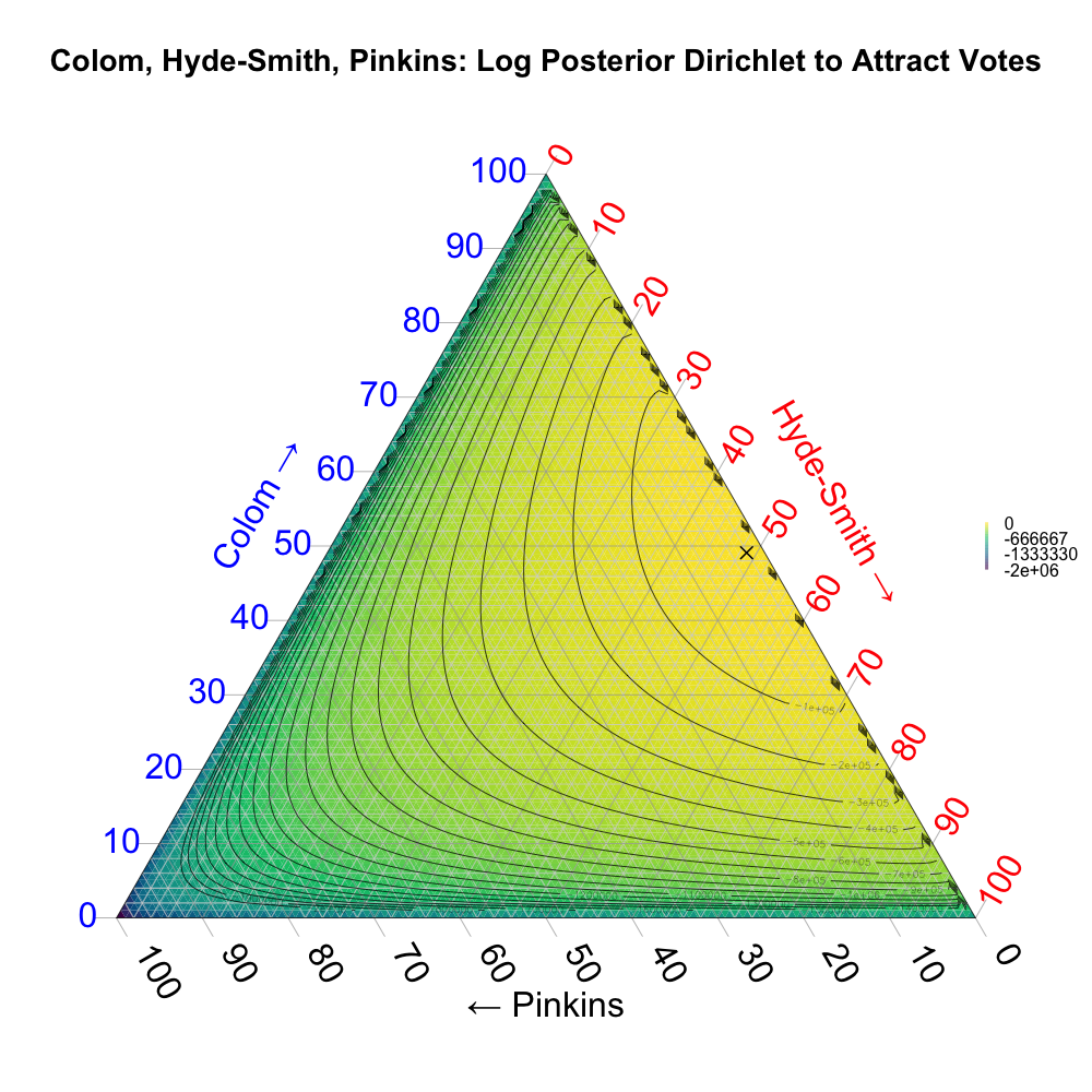We can get an informal idea of the uncertainty here (and more formally below where we concentrate on the 2 major candidates!) by looking at the ternary plot of the Dirichlet distribution, shown here (click to embiggen!).

• The 3 candidates each have an axis on the triangle:
  • Colom’s $p_1$ is along the left edge, increasing upwards.
  • Hyde-Smith’s $p_2$ is along the right edge, increasing downwards.
  • Pinkins’s $p_3$ is along the bottom edge, increasing to the left.
• Note the title says this is log probability!
  • Initially I tried it with straight Dirichlet probability density, but got all kinds of problems since it told me all the values were 0.
    • It turns out the probability is so tightly concentrated around the mode, that any reasonably-sized grid of points will not hit the mod exactly enough to get much probability. In fact, all those probabilities were so small that numerical roundoff rounded them down to 0.
    • Escaping into the land of log-probability fixed this. Since log is a monotone function, none of the minima or maxima are moved, just the shapes are changed.
    • The black spots around the edges are the calculations getting numerically twitchy again at the edges; they’re meaning-free.
• The MAP estimator, the mode of the posterior Dirichlet distribution, is in the center right, marked with an X.
  • Note it is very close to 0% for Pinkins, indicating he has no shot.
  • Note that it is just under 50% for both Colom and Hyde-Smith, indicating what all the anxiety is about.

So the bottom line is: Pinkins has no shot, Colom is slightly ahead of Hyde-Smith, and with this many votes counted we’re pretty sure of that.

Reducing to a 2-Way Election

Suppose we throw out Pinkins as an irrelevancy. Can we quantify the uncertainty between Colom and Pinkins any better?

Yes!

In this case, the multinomial/Dirichlet distributions reduce to binomial/Beta distributions, used many times before on this Crummy Little Blog That Nobody Reads (CLBTNR).

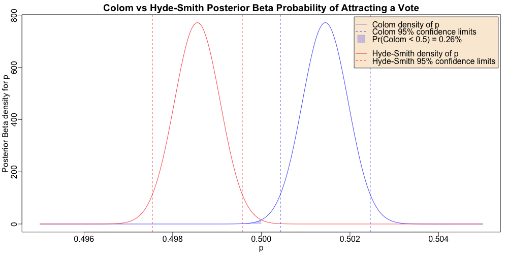Here’s what the posterior distributions for Hyde-Smith (red) and Colom (blue) look like:

• Colom’s median probability of getting a vote is higher than Hyde-Smith’s.
• Not only that, but consider uncertainty: their 95% confidence intervals do not overlap. That means: even in the most optimistic case for Hyde-Smith and the most pessimistic case for Colom, Colom still wins.
• Consider the light blue shading under the left edge of Colom’s curve: that’s the chance his voter-attraction probability is less than 50%, given the election results we see. Note that this says there’s only a 0.26% chance he’s a a loser masquerading as a winner.

Again, the margins are razor-thin, but we’re pretty sure Colom is the winner assuming the remaining absentee/provisional ballots are representative of the rest of the electorate.

The Weekend Conclusion

In a spirit of peer review, everything necessary to reproduce this analysis is available. ^[2]

Mississippi has a well-deserved reputation as a miniature white-supremacist ethnostate within the US. Nevertheless, it has a large Black population. They are now discovering that if they stick together, they can just take over the place.

Good for them.

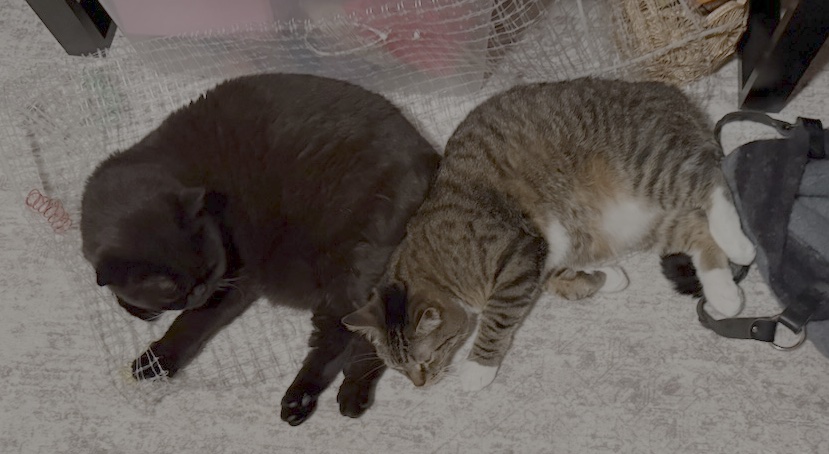All this analysis started out as an exercise in anxiety management on my part. (Hey, don’t judge me. It’s an Elder Nerd thing.)

As you can see, the Weekend Publishers advocate another method of coping. They are asleep on a plastic mesh that pokes them and cannot be comfortable — sort of like a bed of nails for cats. They remind us that not all temporary discomforts are bad.

Wise cats. (Also smartasses, but sure… “wise cats”.)

(Ceterum censeo, Trump incarceranda est!)

(Et ceterum censeo, index Epsteiniani divulganda est!)

---

Notes & References

1: Wikipedia Editors, “2026 United States Senate election in Mississippi”, Wikipedia, downloaded 2026-Nov-10. ↩

2: Weekend Editor, “R script for Bayesian analysis of elections”, Some Weekend Reading blog, 2026-Nov-10.

Also available are:

• A text transcript of everything printed to standard output when running the script.
• An R script with the pipeline-building tools we used.
• An R script with the graphics tools we used.
• A tab-separated values file with the vote counts from Wikipedia that we used.
  ↩